Mixture of Experts (MoE) for Backend Engineers

Suppose a model has dozens of feed-forward subnetworks, but each token uses only two of them. The arithmetic per token can stay modest while the total weight set grows. Now place that model on eight GPUs. If every GPU stores all experts, memory can become the limit; if experts are split across GPUs, token activations must travel to whichever GPU owns their selected experts. What does that trade cost under a real request mix?

This article explains mixture of experts from first principles, then follows its execution across GPUs. We use explicitly constructed examples to show the mechanics. A dense model such as Llama 3.1 70B does not have routed expert layers; its weight and KV calculations must not be transferred to these MoE examples.

A complete MoE layer, step by step

Read this graph from top to bottom. Follow token A in blue and token B in orange through the same layer. Each chooses two experts, yet each produces one combined vector for the next model operation.

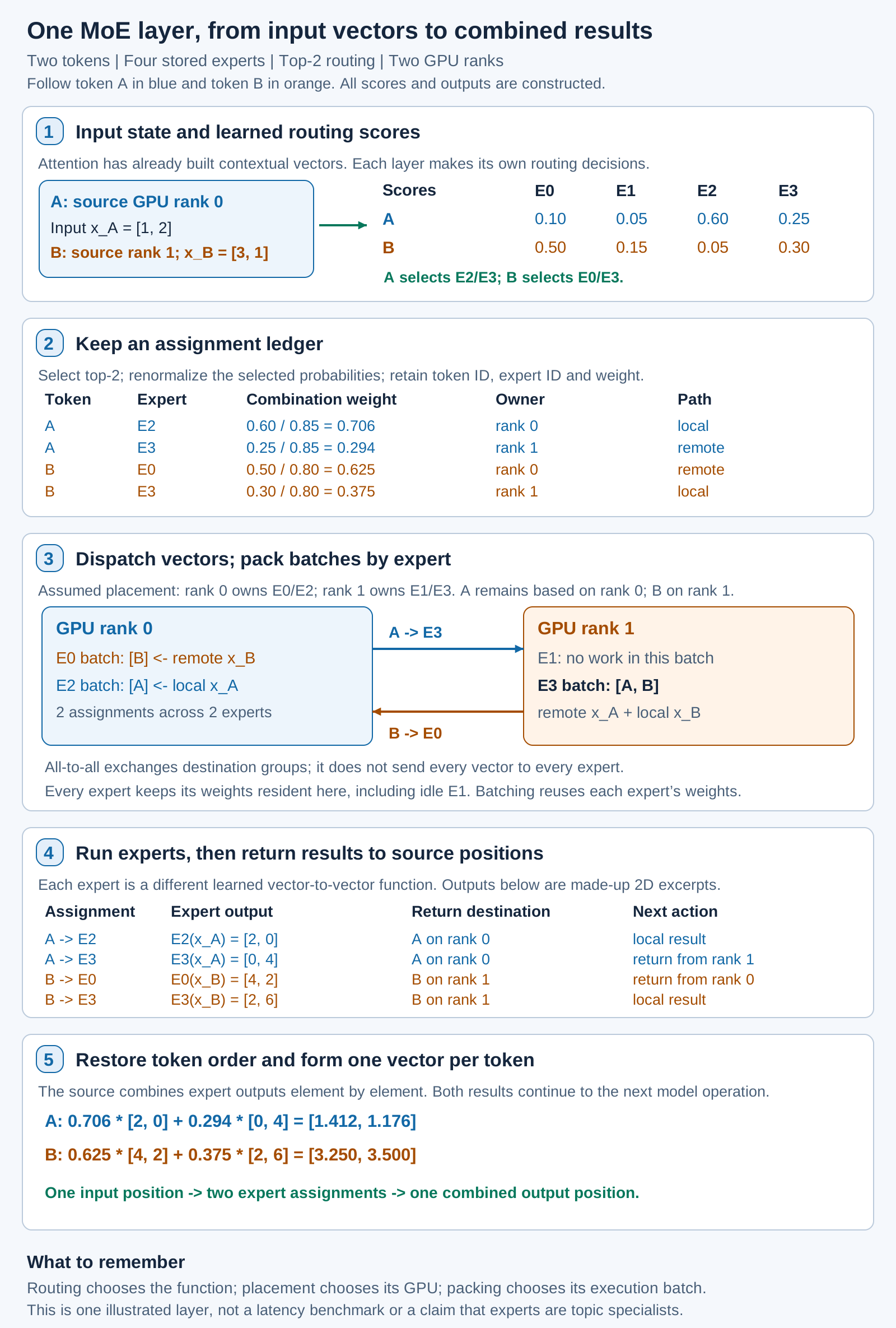
Detailed walkthrough. A constructed two-token batch with four experts and top-2 routing. Rank 0 owns E0/E2; rank 1 owns E1/E3. Output vectors are made-up two-dimensional excerpts and weights are rounded for display. The graph illustrates data movement and arithmetic, not measured latency. Open the full-size graph or its PNG version.

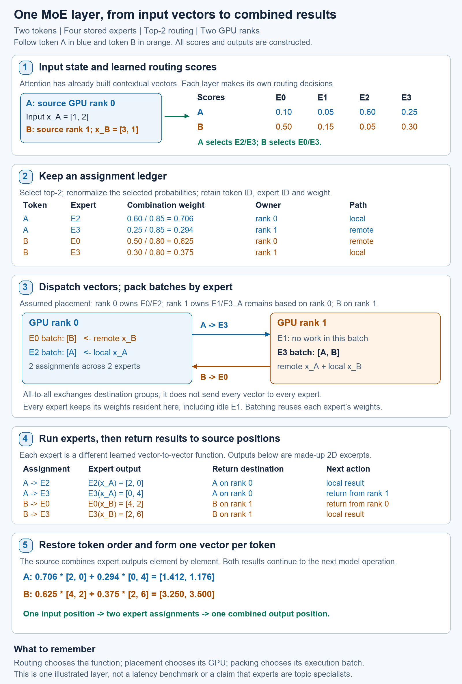
1. Score: each contextual token vector enters the learned router. A chooses E2/E3; B chooses E0/E3.
2. Record: preserve token position, expert ID, destination rank, and combination weight. This ledger lets the runtime regroup work without mixing up results.
3. Dispatch and batch: local assignments stay on their rank; remote assignments cross to their owner. E3 batches A and B together, while E1 is idle in this batch.
4. Return: each selected expert produces a vector. Remote results travel back to the token’s source rank, with assignment metadata identifying where they belong.
5. Combine: scale and sum the expert vectors. A and B each continue as one vector; they do not become two separate generated answers.

The remaining sections unpack why these steps exist, where the worker-pool analogy helps, and which parts of this pipeline constrain serving performance.

What an expert is doing

A model does not pass the string “write some Python” to a Python specialist. A tokenizer first turns text into integer IDs; the embedding layer turns those IDs into vectors of numbers. As a vector passes through Transformer layers, attention incorporates information from visible positions. The hidden state at one position is the resulting contextual vector. MoE routing operates on that vector.

A conventional Transformer layer also contains a feed-forward network (FFN): learned matrix operations and nonlinear functions that transform each position’s vector. Attention mixes information across positions; the FFN transforms each position. In a dense FFN, every token position runs through the same network. A typical sparse MoE sublayer instead offers several FFNs, each with its own learned weights, and runs a selected subset for each position. These FFNs are the experts. Attention can remain dense; a model can also mix ordinary dense FFN layers and MoE layers.

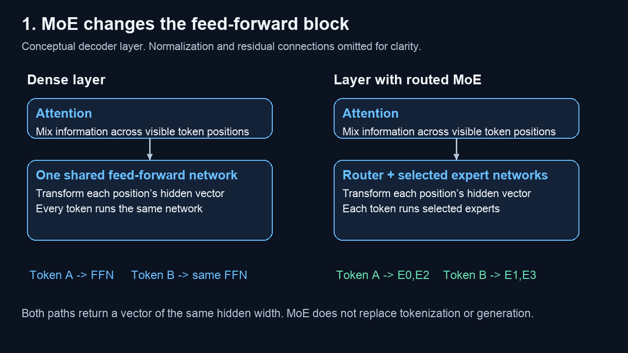
Figure 1. The architectural change is in the feed-forward path. The picture omits normalization and residual connections to focus on that change; experts are networks of weights, not separate chatbots.

Here dense means there is no top-k expert selection in that block. It does not mean every tensor entry is nonzero, every parameter contributes equally, or attention can see future tokens. Sparse refers to conditional expert activation. It does not mean that only a few prompt tokens are processed.

Think of a worker pool with several different implementations of the same vector-to-vector interface. Each implementation accepts an H-element vector and returns an H-element vector, so the next layer can consume the result. This analogy helps explain dispatch and batching. It stops at substitutability: expert E2’s learned function generally differs from E3’s. A serving system cannot substitute the least busy expert for the selected one and expect the same model output.

First, understand what a token executes

An MoE layer contains several experts, typically feed-forward networks, and a learned router. The router scores available experts for each token and selects a small number, often called top-k. With top-2 routing, one token’s activation is sent to two selected experts; their outputs are combined using router weights. Other parts of the Transformer, such as attention, can remain dense and execute for every token. The foundational sparsely gated MoE paper introduced conditional expert computation, while Switch Transformers explored a top-1 design. Neither paper implies every production MoE uses the same k or capacity policy.

The router itself is a learned function, often a small linear projection from the hidden vector to one score per expert. For a Mixtral-style top-2 example, the process is:

1. Score all expert candidates using the token’s current hidden state.
2. Select the two highest scores.
3. Turn the selected scores into combination weights, using the checkpoint’s rule.
4. Run both selected expert networks on the input vector.
5. Add their output vectors element by element, scaled by those weights.

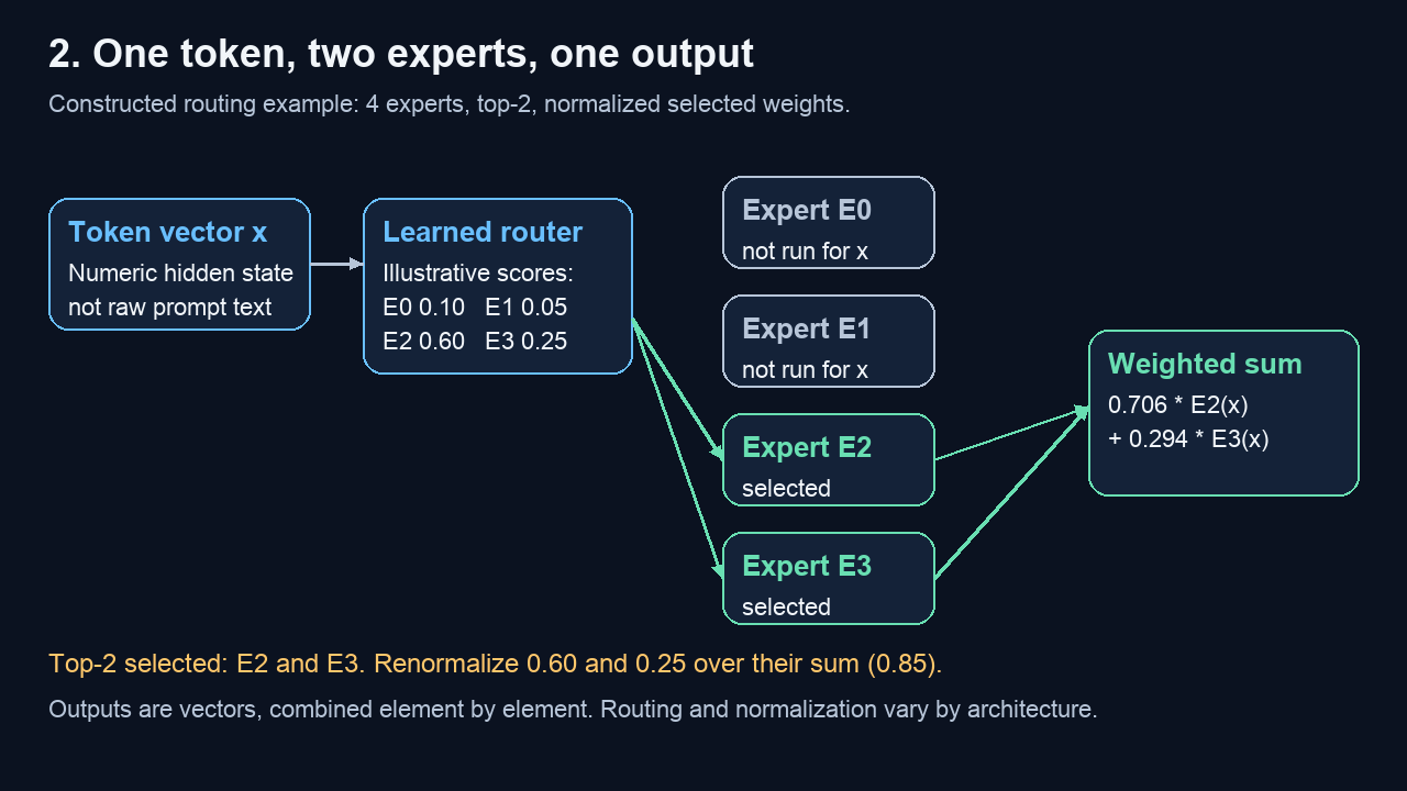
Figure 2. Four candidates keep the picture readable. With illustrative probabilities 0.10, 0.05, 0.60, and 0.25, selecting E2/E3 and renormalizing their weights gives 0.60/0.85 ≈ 0.706 and 0.25/0.85 ≈ 0.294. These numbers are constructed, not a router trace.

If two dimensions of the hypothetical expert outputs are E2(x) = [2, 0] and E3(x) = [0, 4], the combined vector is approximately [1.412, 1.176]. That is a numeric blend, not a vote between two text answers. The Mixtral architecture paper specifies its top-k and weighted-sum rule; other architectures can use different normalization, selected expert counts, or additional shared expert computation, as in DeepSeekMoE. Use the actual checkpoint’s semantics.

The unit of routing is a token position at an MoE layer, not an entire HTTP request. Two tokens in one prompt can choose different experts. The same position can choose different experts at different layers because its hidden state and each layer’s router differ. A request therefore does not acquire one permanent expert for its whole answer.

The name “expert” does not guarantee an English expert, a mathematics expert, or another human topic specialty. Different weights can develop different behavior during training, but topic labels need evidence. Mixtral’s routing analysis found no obvious domain-based pattern in its studied routing distributions. The diagram uses numeric expert IDs deliberately.

Sparse active computation does not mean sparse storage. The server still needs weights for all experts that tokens might select, unless it accepts offloading or loading delays. That is why model fit can motivate expert parallelism even when a token activates only a small fraction of the parameters.

Total parameters, active parameters, and the batch union

For a toy model with equally sized experts and the same k at every routed layer:

P_total  = P_shared + sum_over_MoE_layers(E * P_expert)
P_active = P_shared + sum_over_MoE_layers(k * P_expert)

E = number of routed experts at a layer
k = experts selected per token at that layer
P_expert = parameters in one expert at that layer
P_shared = non-routed parameter component under the counting convention

The distinction describes conditional execution; it is not a literal count of bytes read or floating-point operations. Embedding lookup, shared modules, router work, differing expert sizes, and parameter-count conventions require care. As a named architectural example, Mixtral 8x7B has eight FFN experts per layer, selects two, and reports about 47B total / 13B active parameters. It is not eight complete, independent 7B chat models. Its attention and other components are shared rather than copied eight times. Those are the paper’s model counts, not throughput measurements. Mixtral paper

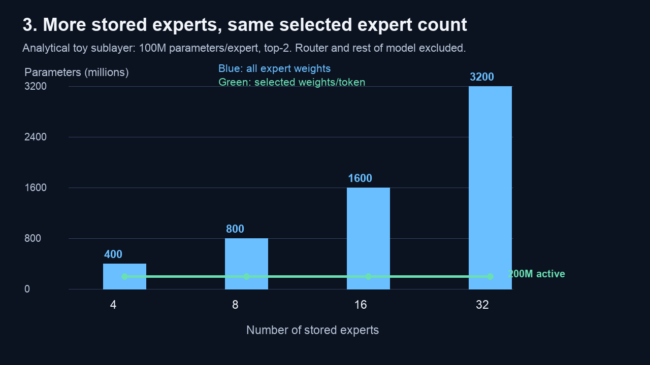
Figure 3. One toy FFN sublayer, 100M parameters per expert, top-2. At E=8, expert storage is 800M parameters (1.6 GB at two bytes/parameter), while one token selects 200M. Router, attention, KV, and runtime buffers are excluded. This is analytical arithmetic, not an actual model or a speedup prediction.

Increasing E at fixed k creates more expert capacity without running all expert networks for each token. It still adds weight storage and may add router/dispatch costs. The server’s resident memory must accommodate experts that later tokens could select, plus shared weights, KV cache, and workspace. Active parameters are a computation clue; total parameters are a weight-capacity clue. Neither determines latency alone.

A batch also changes the memory traffic story. Each token selects k experts, but the union across many tokens can include every expert. A larger batch can reuse each expert’s weights across more vectors, making useful matrix work larger; it can also touch more distinct weights overall. You cannot estimate the batch’s weight reads as one token’s active parameter count multiplied mechanically by batch size.

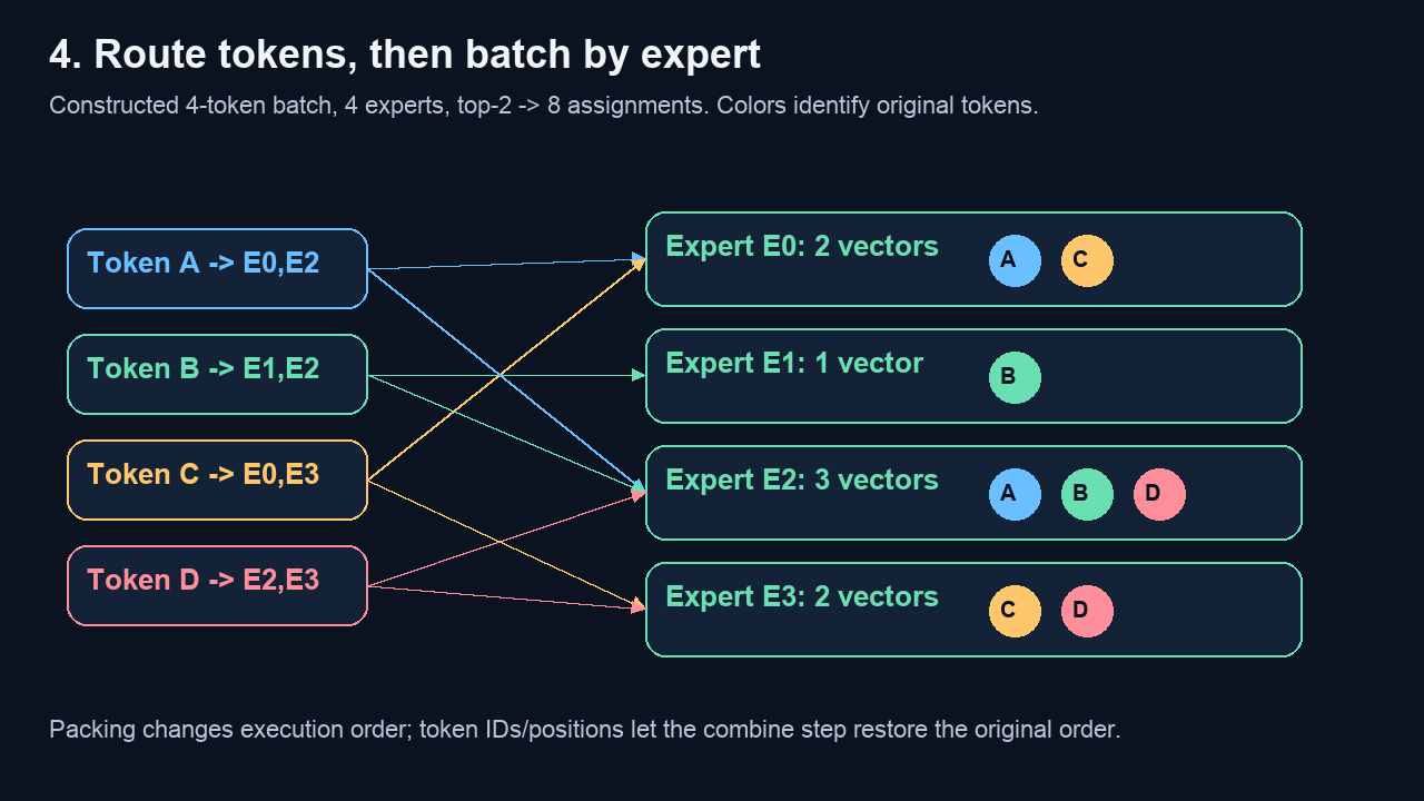
Figure 4. Constructed top-2 routing yields eight assignments from four tokens. E2 receives three vectors; E1 receives one. The runtime packs by expert for efficient computation, then uses assignment metadata to restore each token’s weighted result. Regrouping work does not change the router’s choices.

During prefill, many known prompt positions can contribute assignments to a layer. During ordinary decode, each active sequence contributes one new position per iteration. Low-concurrency decode can therefore leave many experts with tiny batches or no work. High concurrency can improve batching but consumes more KV and can increase queuing. The serving scheduler chooses which requests run; the learned router chooses which expert functions their token vectors use. These are different decisions.

The memory problem and the tempting first design

For a deliberately synthetic example, take 64 experts, top-2 routing, and eight expert-parallel (EP) GPU ranks. A rank is one participating GPU process. If each rank stores all 64 experts, any token can execute locally on the GPU where its other model state sits, avoiding expert dispatch across ranks. But this duplicates expert weights eight times. If the experts alone do not fit in memory, that design is impossible; even when it fits, duplication competes with KV cache and runtime workspace.

Expert parallelism places, initially, eight full experts per rank. The experts are no longer all local to every token. The router’s selected expert IDs decide destinations; the runtime groups token activations by destination, exchanges them, runs local experts, and sends results back. NVIDIA’s TensorRT-LLM expert-parallelism documentation distinguishes this from tensor parallelism, which divides each expert’s weights across GPUs. Hybrid placements can combine both.

Placement of the synthetic 64-expert layer	Expert weights on each rank	New serving cost
Replicate every expert on all eight ranks	64 full experts	Eight copies of expert weights across the group
Place each expert once, split across eight ranks	Eight full experts	Dispatch/return for remote assignments

This is a memory-placement comparison, not a benchmark or a claim that replication is a desirable baseline for every MoE. Attention and other non-expert weights need their own placement, and several modern runtimes support combinations of data, tensor, pipeline, and expert parallel degrees. MoE is a model architecture; EP is an execution placement. An MoE can run without cross-GPU EP if it fits and the runtime supports that configuration.

The two communication phases

Once the router selects top-k experts, an EP implementation typically performs a dispatch exchange: each source rank sends the selected tokens’ hidden-state vectors to the ranks owning those experts. An expert rank groups its received tokens by expert and computes the expert feed-forward networks. A combine exchange returns outputs to their source positions so the runtime can apply router weights and continue the layer. This resembles two all-to-all communication phases, though a particular runtime may implement or overlap them differently. NVIDIA’s NCCL collective guide defines all-to-all as ranks sending different chunks to different peers.

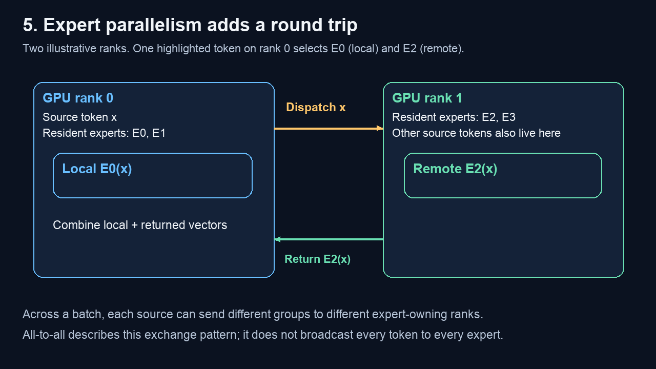
Figure 5. Two ranks make the movement visible. In a full batch, every source can send different destination groups and receive results from several peers. “All-to-all” describes the group exchange pattern, not broadcasting every vector to every expert. Expert execution and exchanges may overlap in a real runtime.

Communication cost depends on where source activations reside, which experts they choose, how tokens are packed, the activation representation, and interconnect topology. A token whose selected expert is local need not cross the network for that assignment. Small batches can make packing and collective launch overhead prominent; large batches carry more bytes. NVLink/NVSwitch within one node and network links across nodes are different paths. The link topology therefore belongs in any performance comparison.

A worked communication bound

Give the synthetic MoE a hidden activation width of 4,096 values, stored as BF16 (2 bytes/value). Process N = 1,024 tokens through one MoE layer with k = 2 selected experts per token. This creates 2,048 expert assignments. Before protocol metadata, padding, or compression, the logical payload sent for one dispatch is:

Dispatch payload = N tokens × k assignments/token × H values/assignment × s bytes/value
                 = 1,024 × 2 × 4,096 × 2 bytes
                 = 16,777,216 bytes = 16 MiB

Dispatch + same-width combine = 2 × 16 MiB = 32 MiB

H is activation width and s is bytes per value; token and assignment units cancel to bytes. 32 MiB is logical payload across the EP group, not measured link traffic or elapsed time. If expert ownership and source placement are independent and balanced across eight ranks, an illustrative remote fraction is 7/8, giving 32 MiB × 7/8 = 28 MiB of cross-rank payload. This is an analytical expectation under that placement assumption. A skewed router, expert replication, topology-aware placement, metadata, padding, or a different combine representation changes it. Do not divide this number by a vendor bandwidth specification and call the result MoE latency; collective startup, contention, expert compute, and synchronization remain.

Memory has a similarly simple first approximation. If each of 64 experts has P parameters at s bytes/parameter and is placed once across eight ranks, expert-weight storage per rank is approximately (64/8) × P × s = 8Ps bytes, before shared weights and buffers. Replicating all experts on every rank would require 64Ps bytes per rank. This explains the fit benefit, not the total model footprint or whether EP beats a tensor-parallel alternative.

The slowest rank sets the pace

The average assignment count in this example is 2,048 / 8 = 256 assignments/rank. That average can hide a hot rank. Imagine the following constructed distribution; it is not an observed router trace:

Rank	0	1	2	3	4	5	6	7
Even assignment count	256	256	256	256	256	256	256	256
Skewed assignment count	640	320	256	224	192	160	144	112

The skewed counts still sum to 2,048, but the busiest rank has 640 / 256 = 2.5 times the average work by assignment count. Actual time need not be 2.5 times longer: experts may have different kernels, padding, or overlap, and communication can dominate. The graph makes only the imbalance visible.

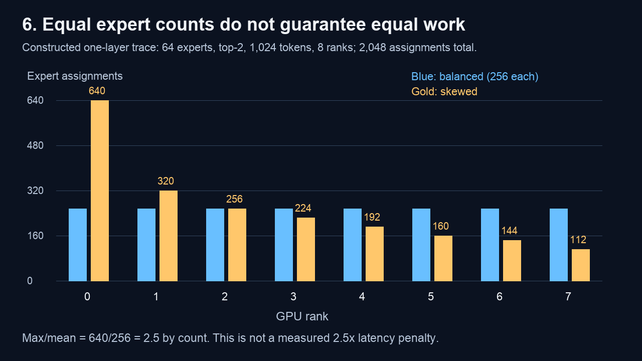
Figure 6. Counts, not timings. Rank 0 carries 640 assignments while the mean is 256. Equal numbers of resident experts do not imply equal load.

An MoE layer often cannot complete until routed outputs return. Hot experts can therefore stall other ranks and create tail latency even when total GPU utilization appears high. A naive response is to give every rank the same number of experts, but equal expert counts do not imply equal token counts. Possible remedies include moving hot experts, replicating selected experts, changing the routing policy during model design, or adding capacity headroom. Replication spends memory; remapping and routing spend control effort and can alter locality. vLLM’s expert-parallel deployment guide documents an expert-parallel load balancer that redistributes mappings when observed expert loads are skewed.

Some MoE architectures impose a capacity per expert or an overflow policy. Depending on the design, overflow assignments can be dropped, rerouted, or processed through a different scheduling strategy. Training capacity rules should not be assumed to describe inference behavior. This is not a harmless serving knob: changing which experts a token uses can change model output quality. Distinguish placement-only changes, intended to preserve the same expert computation, from changes to top-k routing, capacity, precision, or overflow. Even placement-only changes need numerical-equivalence checks because floating-point execution order and kernel choice can vary.

When EP helps, and when it hurts

EP is attractive when all expert weights cannot be replicated within memory, when routing has enough tokens to batch local expert work, and when the interconnect can move routed activations without dominating the step. It can also make better use of several GPUs for a large MoE. It may perform poorly at tiny decode batches, with severe expert skew, across slow inter-node links, or when an alternative tensor/replica placement already meets the SLO. Higher total model parameter count does not by itself predict speed, because only selected experts execute but all expert weights must be placed somewhere.

For user experience, dispatch and combine can add to time to first token (TTFT) during prefill and inter-token latency (ITL) or TPOT during decode. More capacity may improve request throughput or reduce queues, but extra synchronization can worsen P95/P99. KV memory still belongs to active sequences and competes with expert weights. The hardware bill includes all EP ranks plus network capacity, spare capacity for hot experts, and redundancy. Compare cost per SLO-compliant request, not nominal tokens per second alone.

Reliability changes too. A request whose token needs an expert on a failed rank cannot simply use a different surviving expert without changing computation. A deployment needs replica groups, retry/recovery policy, and admission behavior for rank failures. Cross-node EP widens the failure and network domain. Monitor rank health and collective errors as well as latency.

Production implementation and a fair test

vLLM’s current EP documentation explains its deployment choices, all-to-all backends, and load-balancing options. TensorRT-LLM documents EP versus expert tensor parallelism and hybrid configuration. These examples illustrate placements, not a universal performance ordering; pin the runtime and model revisions before citing exact flags or behavior. NCCL supplies communication primitives that can underlie such exchanges, although a runtime may use a specialized backend.

First simulate uniform and skewed top-2 routing to understand expected assignments/rank and remote payload. Then benchmark an actual named MoE model under at least two supported placements with the same checkpoint, tokenizer, precision, expert routing, GPU count, topology, runtime version, input/output distribution, concurrency, sampling, scheduler budgets, warm-up, duration, and repetitions. Include low-concurrency chat and high-throughput batches. Measure per-rank assignment count, expert compute time, dispatch/combine time and bytes, GPU memory, queue time, TTFT and ITL/TPOT P50/P95/P99, output tokens/s, SLO goodput, output-quality equivalence, and cost. Capture traces to see whether the critical path is expert compute, a hot rank, or communication. Do not compare EP results from one MoE with dense Llama throughput as if architecture were held constant.

Investigate EP when expert weights or replicated placement strain memory, or traces show expert work could be distributed. Keep the placement when model fit and measured SLO goodput improve after accounting for all-to-all, skew, quality, and failure handling. Once tensor shards or experts span GPUs, communication itself may dominate. Inspect the actual collective trace and link topology before increasing the expert-parallel group.

Engineering checklist

Engineering question	EP answer to verify
Problem, symptoms, measurement, root cause	Expert-weight memory or hot-rank stalls; measure memory, per-rank assignments, collective time, TTFT/ITL tails.
Naive fix, optimization, mechanism	Equal expert counts alone miss skew; place different experts on ranks and dispatch only selected tokens.
Architecture, GPU, memory	Router → exchange → local expert kernels → return/combination; fewer expert weights per rank, added buffers and fabric traffic.
Performance, quality, cost	Fit and goodput may improve; tails can worsen; placement should preserve routing, while capacity/precision changes can alter quality; ranks and links cost money.
Best/poor workloads, trade-offs	Large MoE with adequate batch/fabric / tiny batches, skew, slow network; replication buys balance with memory.
Implementation, benchmark, interactions, decision	Pin vLLM or TensorRT-LLM, compare same MoE and topology; account for TP/PP, quantization, scheduling, and communication.

References

• Jiang et al., Mixtral of Experts, especially architecture and routing analysis, for a concrete top-2 model and total versus active parameter counts.
• Dai et al., DeepSeekMoE for a design with shared and routed expert components.
• Shazeer et al., sparsely gated MoE and Fedus et al., Switch Transformers for conditional expert computation and routing variants.
• vLLM expert-parallel deployment guide for current placement, communication, and balancing options.
• NVIDIA TensorRT-LLM expert-parallelism guide for EP, expert TP, and hybrid placement.
• NVIDIA NCCL collective operations for all-to-all semantics.

Primary sources and runtime documentation checked on 2026-09-25. This article provides analytical and constructed examples; it contains no measured GPU benchmark. All diagrams are static; the full-size walkthrough is available in SVG and PNG above.

Key takeaways

• MoE sparsity limits active expert computation per token, while all expert weights still need placement.
• EP distributes expert weights and adds dispatch/combine traffic. The busiest rank and fabric can set layer latency.
• Equal expert counts do not ensure balanced token loads; evaluate placement using per-rank traces and P95/P99.
• A valid comparison holds the MoE model and routing fixed and tests quality, SLO goodput, memory, network, cost, and failure behavior.