Distributed LLM Inference: TP, PP, and EP Explained

Suppose you have a language model and eight GPUs. What should each GPU do?

One answer is to give every GPU a complete copy of the model and send each copy different requests. Another is to make several GPUs cooperate on the same model. But even then, “split the model” leaves a question unanswered: split what?

That question separates three ideas:

• Tensor parallelism (TP): split the calculations inside a layer.
• Pipeline parallelism (PP): split the sequence of layers into stages.
• Expert parallelism (EP): place different experts of a Mixture of Experts model on different GPUs.

We’ll follow the data through each arrangement. By the end, you should be able to look at a GPU layout and explain what each device owns, what it computes, and why it needs to communicate.

All small matrices, routing choices, and timing examples below are constructed for teaching. They are not benchmark results.

1. Why use more than one GPU?

Start with a practical obstacle: the model might not fit.

A model with roughly 70 billion parameters, such as Llama 3.1 70B, needs approximately this much memory for BF16 weights:

70 billion parameters × 2 bytes per parameter = 140 GB

Here, GB means decimal gigabytes. An H100 SXM has 80 GB of GPU memory, so one cannot hold those weights entirely in its memory at that precision. This example assumes resident BF16 weights; quantization and offloading change the problem.

Even two GPUs are not automatically enough for a usable deployment. Dividing 140 GB by two gives an ideal 70 GB of weights per GPU, but serving also needs the KV cache, temporary activations, and runtime buffers. Weights are only part of the memory budget. The KV cache article explains the request state that grows as tokens accumulate.

More GPUs can therefore serve three purposes:

Goal	What extra GPUs provide
Fit a large model	More memory across devices, with the model partitioned appropriately
Finish a model step sooner	More devices doing useful work on that step, if coordination costs allow
Serve more independent requests	Additional complete serving instances

These goals can overlap, but they are different. Fitting the weights across eight GPUs does not imply an eightfold speedup.

2. The picture to keep in mind

A Transformer processes numerical representations through a stack of layers. Each layer includes attention and a feed-forward network. During generation, the model runs through the stack to produce scores for the next token, selects a token, and repeats.

A hidden state is the vector of numbers representing a token position at a particular point in that computation. An activation is an intermediate value produced by the network. When a pipeline stage sends an activation, or an MoE router dispatches a token, it is these numerical representations that move between GPUs.

Now imagine cutting this computation in three different places.

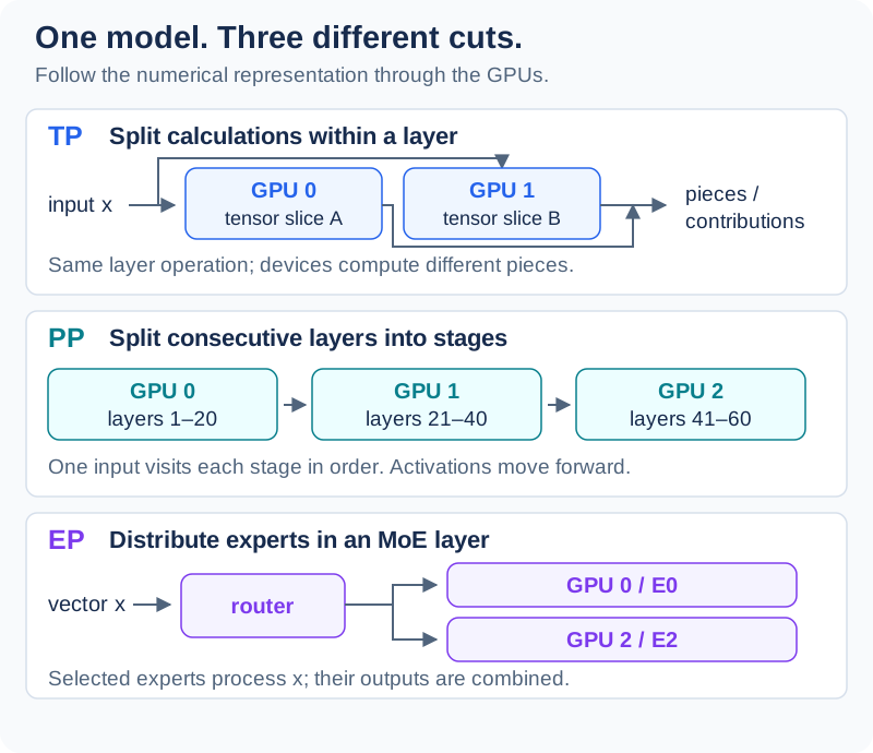
TP divides work within a layer. PP divides the layer stack. EP distributes the expert networks inside an MoE layer. The drawings show ownership and dependencies; they are not timing diagrams.

The useful question is always: what must happen before this token representation can continue?

3. Tensor parallelism: several GPUs work inside the same layer

Imagine a layer containing a large matrix multiplication:

input vector × weight matrix = output vector

The weight matrix can be too large, or the multiplication too expensive, for one GPU. TP partitions that operation so several GPUs compute pieces of it.

Split the output into pieces

Use a tiny example with input x = [2, 3] and a matrix W with two rows and four columns:

          columns 0–1   columns 2–3
W =       [ 1   0    |   1   2 ]
          [ 0   1    |   1   1 ]

Split W by columns. GPU 0 stores the left half; GPU 1 stores the right half. Both have the input x.

GPU 0: [2, 3] × [1  0] = [2, 3]
                [0  1]

GPU 1: [2, 3] × [1  2] = [5, 7]
                [1  1]

Together, the two results represent the full output:

y = [2, 3 | 5, 7]

Each GPU computed different output coordinates of the same operation. Neither calculated the whole output by itself.

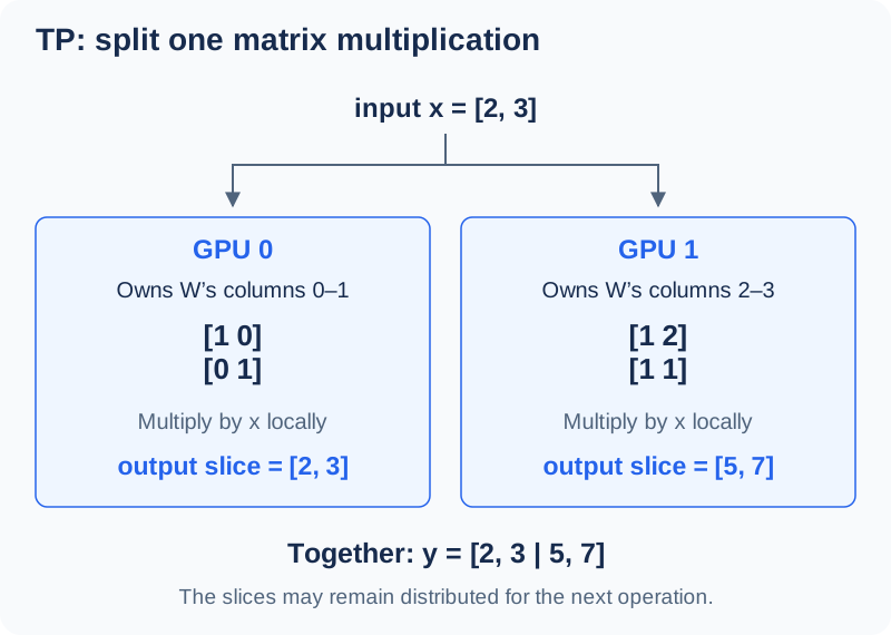
A column split produces output slices. They can stay distributed if the next operation accepts them; assembling the full vector everywhere would require an all-gather.

Sometimes the pieces must be added

Now suppose the next projection takes our four-value output and produces one number:

z = [2, 3, 5, 7] · [1, 2, 3, 4]
  = 2 + 6 + 15 + 28
  = 51

The input is already split, so give each GPU the matching weights:

GPU 0: [2, 3] · [1, 2] =  8
GPU 1: [5, 7] · [3, 4] = 43

combine: 8 + 43 = 51

Here, each GPU owns a partial sum for the same output, rather than a different output slice. Concatenating [8, 43] would be wrong. The contributions must be added. A sum all-reduce can do this and leave 51 on both GPUs.

This explains two common TP communication operations:

• All-gather: collect different slices into a complete tensor.
• All-reduce: combine contributions, such as partial sums, and distribute the combined result.

These are different operations, as defined in NVIDIA’s NCCL documentation.

The pairing in our example is useful: the first multiplication produces distributed slices, and the second consumes those slices directly. There is no need to assemble the intermediate vector first. The Megatron-LM paper applies this pattern to Transformer feed-forward blocks using column and row partitions. It also partitions attention work across heads. Real layers include nonlinearities, normalization, residual paths, and sometimes gated projections; our arithmetic isolates the partitioning idea.

What TP buys, and what it costs

With TP = 4, four GPUs cooperate on partitioned operations within a layer. They continue cooperating as execution moves through the model. Large weight tensors are divided, although some smaller tensors or operations may be replicated.

TP can reduce the memory and arithmetic assigned to each GPU. The price is repeated communication during layer execution. Smaller local calculations may finish sooner, yet still wait for the other GPUs and their results.

Think of four people calculating different parts of the same spreadsheet. They can work concurrently, but formulas that depend on everyone’s results create coordination points.

TP’s defining dependency: a layer needs the appropriate pieces or combined contributions before dependent work can continue.

4. Pipeline parallelism: each GPU owns a stretch of layers

PP makes a different cut. It keeps consecutive layers together and assigns each group to a stage.

For an illustrative 80-layer model with four stages:

GPU 0           GPU 1           GPU 2           GPU 3
layers 1–20  →  layers 21–40  →  layers 41–60  →  layers 61–80

GPU 0 processes the input using its layers, then sends the resulting activations to GPU 1. GPU 1 applies its layers and sends its output onward. The weights normally stay with their stages.

One input still traverses all four stages in order. GPU 3 cannot finish its portion before GPU 2 produces the required input.

Where does the parallel work come from?

An assembly line becomes busy when different stations work on different items. A model pipeline works similarly: different stages process different microbatches, or small groups of inputs scheduled through the pipeline.

To see the timing clearly, use a separate toy pipeline with three stages. Assume every stage takes exactly 10 ms, and ignore transfers and scheduling overhead. A, B, C, and D are four independent input groups.

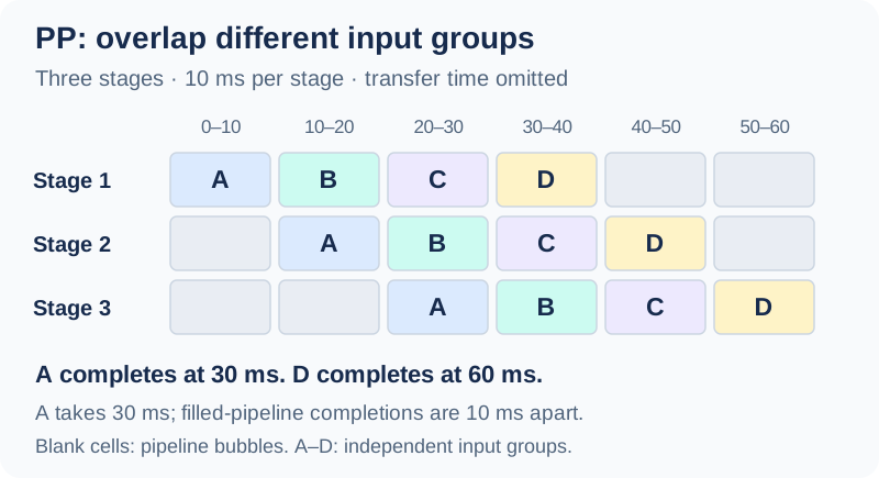
In slot 3, stage 1 processes C, stage 2 processes B, and stage 3 processes A. Blank cells are idle slots, often called pipeline bubbles.

Follow A across the diagonal: it takes three slots, or 30 ms, to complete. Once the pipeline fills, a different group completes every 10 ms. All four groups finish after six slots, or 60 ms.

Without overlap, sending A all the way through before starting B would take 4 × 30 = 120 ms for the same four groups. Pipelining improves the rate of completed groups in this constructed example. A still passes through three sequential stages.

The GPipe paper develops layer partitioning and microbatch pipelining for training. Our diagram uses only forward execution to illustrate the dependency relevant to inference.

Generation has an extra dependency

For one ordinary autoregressive sequence, the next generated token depends on the token just selected at the end of the previous pass. It cannot simply start its next full decode pass while that token is still unknown.

That makes independent requests valuable for filling an inference pipeline. A single request generating one token at a time provides less independent work than several requests or appropriately scheduled input groups. Prefill and decode also have different amounts of work; a serving runtime’s schedule determines how much overlap is possible.

PP therefore offers a clear way to spread layers and their weights across devices, but it can leave devices idle when there is too little concurrent work. An unusually slow stage also limits the completion rate. Equal layer counts are a starting point, not a guarantee of equal execution time.

PP’s defining dependency: an input must finish one stage before entering the next; parallelism comes from overlapping different inputs.

5. Expert parallelism: send each token to the GPUs holding its experts

EP needs a model with Mixture of Experts (MoE) layers. A dense model such as Llama 3.1 70B does not have routed experts to distribute. We’ll switch to a toy MoE model here.

An MoE layer offers several feed-forward networks called experts. A router selects a few for each token representation. Each selected expert transforms that vector, and their outputs are combined. If this is new, the visual MoE guide walks through the architecture.

EP answers a placement question: which GPU stores each expert? In a simple EP-only layout, each GPU owns complete experts. TensorRT-LLM’s guide contrasts this with TP, which can split each expert’s weight tensors across GPUs.

Follow one token across devices

Suppose one MoE layer has four experts:

GPU	Expert weights stored there
GPU 0	E0
GPU 1	E1
GPU 2	E2
GPU 3	E3

Token A’s current vector x is on GPU 0. Its router selects E0 and E2, with combination weights 0.7 and 0.3.

1. Dispatch: keep x locally for E0 and send a copy to GPU 2 for E2.
2. Compute: GPU 0 evaluates E0(x); GPU 2 evaluates E2(x).
3. Return: send E2’s output back to GPU 0 in this simple layout.
4. Combine: compute 0.7 × E0(x) + 0.3 × E2(x) so one vector can continue.

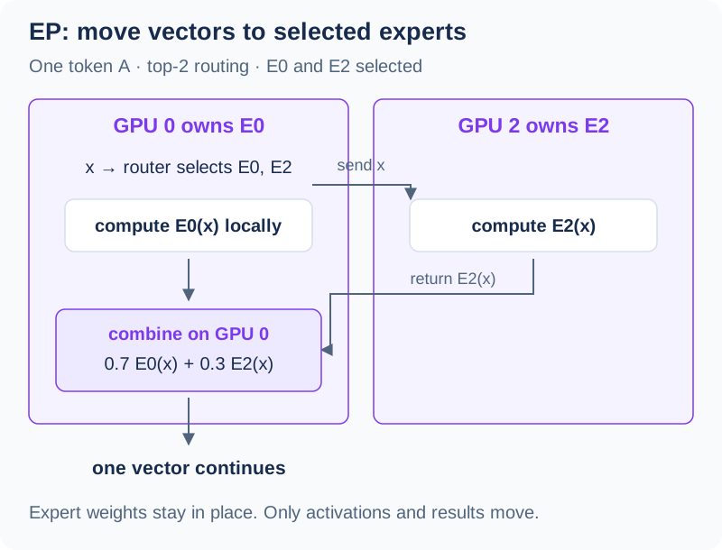
Only the selected experts process A. GPU 1 and GPU 3 may process other tokens. The arrows carry activations and results; expert weights stay on their owning GPUs.

For example, if E0(x) = [2, 0] and E2(x) = [0, 4], then:

combined output = 0.7 × [2, 0] + 0.3 × [0, 4]
                = [1.4, 1.2]

The layer has two expert assignments for A, followed by one combined output. A was not permanently assigned to E0 or E2: another token, or the same position at another MoE layer, can take a different route.

A batch turns routing into a traffic pattern

Now add three more token vectors:

A → E0, E2
B → E1, E2
C → E0, E3
D → E2, E3

There are eight assignments: four tokens times two selected experts. Group them by destination:

GPU 0 / E0: A, C       2 assignments
GPU 1 / E1: B          1 assignment
GPU 2 / E2: A, B, D    3 assignments
GPU 3 / E3: C, D       2 assignments

Every token uses only two experts, but the batch uses all four. GPU 2 receives more expert work than GPU 1. If its queue is slow to finish, dependent combinations must wait for its outputs.

With input vectors originating on multiple GPUs, dispatch becomes a many-to-many exchange: each device may send different vectors to several destinations. This is an all-to-all communication pattern. The return phase sends results toward their combination locations. Implementations can realize these exchanges using different primitives; vLLM’s EP guide documents multiple communication backends and expert load balancing.

EP distributes expert storage and work, but routing creates communication and potentially uneven queues. It also does not determine the placement of attention and other shared components; those need their own arrangement.

EP’s defining dependency: a token needs the outputs of its selected experts, wherever those experts live, before combination can finish.

6. Compare the three cuts

	TP	PP	EP
What is divided?	Tensors and operations within layers	Consecutive layers	Experts within MoE layers
What does one GPU own?	Slices of large weight tensors	Weights for its stage	A subset of experts, in the simple EP-only case
What happens to one token?	GPUs calculate pieces of the same layer operation	Its representation visits stages in order	Its representation visits selected experts
Where does parallel work come from?	Pieces of one operation execute concurrently	Different inputs occupy different stages	Different expert assignments execute concurrently
Characteristic communication	Exchange slices or combine partial contributions	Send activations to the next stage	Dispatch vectors and return expert outputs
Typical difficulty	Frequent synchronization	Idle bubbles or a slow stage	Routing traffic or overloaded experts

TP and PP can apply to dense or MoE Transformers, subject to runtime support. EP applies to models with experts. These are descriptions of computation and placement, not promises about speed.

7. Can they be combined?

Yes. A pipeline stage can itself contain a TP group.

For a dense model, TP = 2, PP = 2 gives one model instance across four GPUs:

Stage 1: earlier layers              Stage 2: later layers
┌────────────────────────┐          ┌────────────────────────┐
│ GPU 0 + GPU 1          │ ───────→ │ GPU 2 + GPU 3          │
│ tensor-parallel group  │          │ tensor-parallel group  │
└────────────────────────┘          └────────────────────────┘

Within each stage: GPUs cooperate on tensor operations.
Between stages:    activations move forward through the layers.

Each GPU stores tensor slices for the layers in its own stage. It does not store a tensor slice of every layer in the entire model.

For a dense deployment with independent TP and PP dimensions:

GPUs per complete model instance = TP × PP

vLLM supports combining TP and PP. One useful placement is TP among GPUs connected by fast local links and PP between groups, so frequent TP exchanges stay local. Whether it works well depends on the actual topology and workload.

For MoE models, expert ownership can also be partitioned, and an individual expert can itself use TP. But do not automatically multiply TP × PP × EP to count GPUs. Runtimes can reuse the same devices for different parallel groups. For example, vLLM derives its EP group size from its TP and data-parallel sizes; EP is not an extra independent device multiplier in that arrangement.

8. A replica is a complete model instance

A shard is one piece of a model. A replica is a complete serving instance, even when that instance spans several GPUs.

With eight GPUs, two possible layouts are:

One TP8 instance:
  request A → [GPUs 0–7 cooperate on one model]

Two TP4 replicas:
  request A → [GPUs 0–3 cooperate on model copy 1]
  request B → [GPUs 4–7 cooperate on model copy 2]

Both layouts can handle batches; the distinction is the number of independent complete instances. The TP8 instance can batch A and B together. The two TP4 replicas can run separate batches without an eight-GPU tensor collective joining their layer calculations.

For our approximate 140 GB of BF16 weights, the ideal weight share is 17.5 GB per GPU with TP8, or 35 GB per GPU inside each TP4 replica. Two replicas store two complete weight copies overall. These are weight-only arithmetic estimates; neither establishes a safe context length or concurrency limit.

Adding a replica can increase independent serving capacity. Increasing TP instead changes how devices cooperate on each instance. Those choices can have different effects on per-request latency and total throughput.

9. Why more GPUs can still mean more waiting

Every GPU has local memory. A value computed on GPU 0 does not instantly appear on GPU 1. The devices need links, transfers, and coordination.

The three strategies expose three kinds of waiting:

• TP: “My partial calculation is finished, but I need the other contributions.”
• PP: “My stage is ready, but the previous stage has not sent this input.”
• EP: “One selected expert has finished, but another selected expert’s result has not returned.”

For intuition, suppose one operation takes 10 ms on one GPU. An ideal two-way split reduces local work to 5 ms. If the split adds 1 ms of communication that cannot overlap, the step takes 6 ms. If it adds 6 ms instead, the step takes 11 ms. This invented arithmetic illustrates the tradeoff; real execution includes overlap and more dependencies.

Large transfers need bandwidth. Small, repeated exchanges can be limited by launch and synchronization latency. A fast link helps, but it does not remove the need to wait for required inputs. This connects directly to the memory and execution model in GPU 101 for Backend Engineers.

When you see a distributed inference layout, trace one token representation:

1. Which weights are local to each GPU?
2. Which operations can run at the same time?
3. Which numerical values must cross devices?
4. Which missing result would stop the next operation?

Those questions turn the abbreviations into concrete execution paths: TP shares a layer’s calculation, PP hands work through layer stages, and EP routes work to selected experts. Replicas add more complete paths for independent requests.

---

Further reading

• Megatron-LM: column and row partitioning inside Transformer layers.
• GPipe: layer partitioning and microbatch pipelines, developed for training.
• TensorRT-LLM expert parallelism: expert ownership versus tensor slices, including hybrid layouts.
• NCCL collective operations: all-gather, all-reduce, and all-to-all semantics.
• vLLM parallelism and scaling, and expert parallel deployment: how serving runtimes expose these ideas.

Adapted from my distributed inference fundamentals notes. The small worked examples and diagrams are original teaching illustrations. Technical sources checked on October 7, 2026.