Mixture of Experts: A Bigger Brain Without Using All of It

How a token chooses a few neural networks, blends their outputs, and keeps moving.

All small numerical examples are invented for explanation.

Imagine a wall of eight switches. Each switch powers a different neural network.

A token arrives. Two switches light up. Those two networks do their work; the other six stay idle for this token. Another token arrives, and a different pair lights up.

Now imagine adding another eight switches to the wall. You have doubled the number of networks available, but each token still turns on only two.

That is the central idea behind sparse Mixture of Experts, or MoE: give a model more learned functions to choose from while limiting how many it evaluates for each input. This is conditional computation, developed in the sparsely gated MoE work.

The appealing part is easy to see. The subtle part is what the switches actually control. To understand that, let’s follow one token.

1. Start with a vector, not a word

Consider this sentence:

The fisherman sat on the bank.

Inside a language model, “bank” is represented by numbers. A token is a piece of text; its hidden state is the vector the model is currently using to represent that position. For our picture, imagine a short arrow. In a real model, it has many more coordinates.

Attention lets that position gather information from visible positions, including clues such as “fisherman.” A feed-forward network then transforms the resulting vector, independently at each position. These two operations alternate through Transformer layers. Transformer paper, §§3.2–3.3

One way to picture an ordinary feed-forward network is a workshop: expand the vector into a larger set of features, apply a nonlinear transformation, and project back to the original width. A simple version looks like:

input vector → expand → nonlinear transformation → project back

The same workshop processes every token position. Its output depends on the input, even though its weights are shared across positions. The original Transformer uses this kind of position-wise network; later models often use gated variants. Transformer paper, §3.3

MoE changes the workshop arrangement.

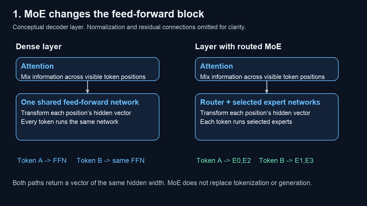
Both paths transform a token vector. Normalization and residual connections are omitted to keep the architectural change visible.

2. Replace one workshop with several

An MoE layer offers several feed-forward networks, each with its own learned weights. These are the experts. A small learned network, the router, selects which ones will process the current vector.

Each expert accepts a vector and produces another vector of the required width. That common shape makes their outputs combinable, while their different weights let them learn different transformations. The foundational MoE paper describes a sparse gate over expert subnetworks. Shazeer et al.

Pause at the name “expert.” It is tempting to draw a math professor, a programmer, and a poet behind those switches. That picture can mislead. The name describes a learned subnetwork; any recognizable specialization has to be established from evidence. Mixtral’s analysis found no obvious separation by topic in the domains it examined, and observed patterns associated with syntax. Mixtral routing analysis

For our drawings, we’ll use neutral labels: E0, E1, E2, and E3.

3. Follow one token through the router

Suppose our token’s contextual vector is called x. Our toy layer has four experts and chooses two, a rule called top-2 routing.

The router produces scores. For this example, after converting them to probabilities, we get:

Expert	Router probability	Selected?
E0	0.10
E1	0.05
E2	0.60	Yes
E3	0.25	Yes

E2 and E3 have the highest values, so only they run for x.

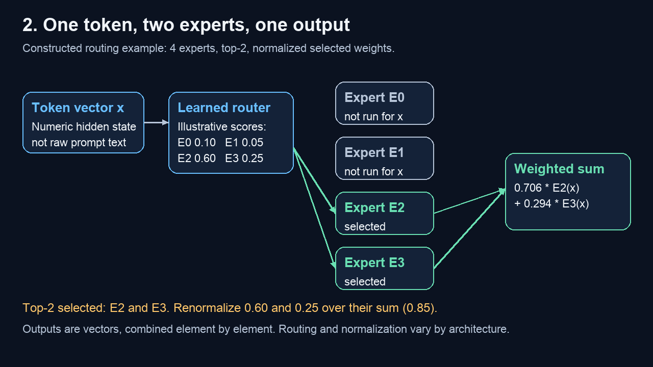
Constructed example: four candidates, two selected experts. The selected probabilities are renormalized before combining outputs.

We need two things from the router: which experts to execute, and how strongly to weight their results. In our example, the selected probabilities sum to 0.85. Dividing by that sum gives:

E2 weight = 0.60 / 0.85 = 12/17 ≈ 0.706
E3 weight = 0.25 / 0.85 =  5/17 ≈ 0.294

The two weights now sum to one. This matches the selected-score softmax rule described for Mixtral. Other MoE designs can use different gating and normalization rules. Mixtral architecture, §2.1

For a common linear router, the score for an expert is a dot product between x and a learned vector associated with that expert. Geometrically, each candidate tests a different direction in the hidden-state space. The router learns those directions; a high score is a routing preference, rather than a calibrated guarantee that the expert is correct. Jia-Bin Huang’s visual explanation, 9:02–9:33

Routing uses the current contextual vector. A word in a different sentence, or its representation at another layer, may take a different route.

4. Two outputs become one arrow

Now make the expert outputs small enough to draw:

E2(x) = [2, 0]     an arrow pointing right
E3(x) = [0, 4]     an arrow pointing up

Scale the first arrow by 12/17. Scale the second by 5/17. Then add them:

y = (12/17) × [2, 0] + (5/17) × [0, 4]
  = [24/17, 20/17]
  ≈ [1.412, 1.176]

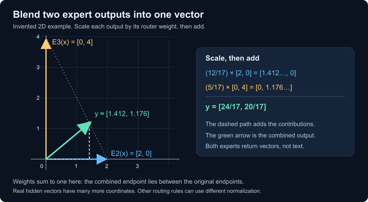
The dashed path adds the two scaled contributions head to tail. Because this example uses nonnegative weights summing to one, y also lies on the segment between the original expert outputs. These axes are numerical coordinates, not named concepts.

Open the scalable vector diagram.

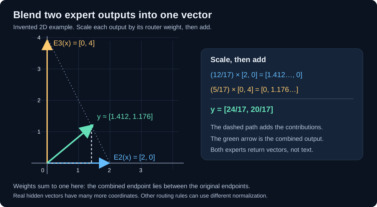
This is what the “mixture” looks like: two transformations contribute to one new representation. The full model continues processing that representation before producing next-token scores.

The general expression is compact:

\[y = \sum_{i\in S(x)} g_i(x)\,E_i(x).\]

Here, S(x) is the selected set of experts, Eᵢ(x) is an expert’s output, and gᵢ(x) is its combination weight. The formula says exactly what our arrows did: select, scale, add.

In a typical Transformer block, the MoE output is added back to the residual stream, the running token representation. Our y denotes the expert mixture alone; the entire block includes that residual connection and other operations. DeepSeekMoE architecture

5. Bigger capacity, bounded expert work

Return to the wall of switches. What happens if we add more experts but keep selecting two?

Assume each expert in one toy layer contains 100 million parameters. Ignore the router and the rest of the model for a moment.

Available experts	Stored expert parameters	Selected expert parameters per token
4	400 million	200 million
8	800 million	200 million
16	1.6 billion	200 million
32	3.2 billion	200 million

The first numeric column grows. The second stays still.

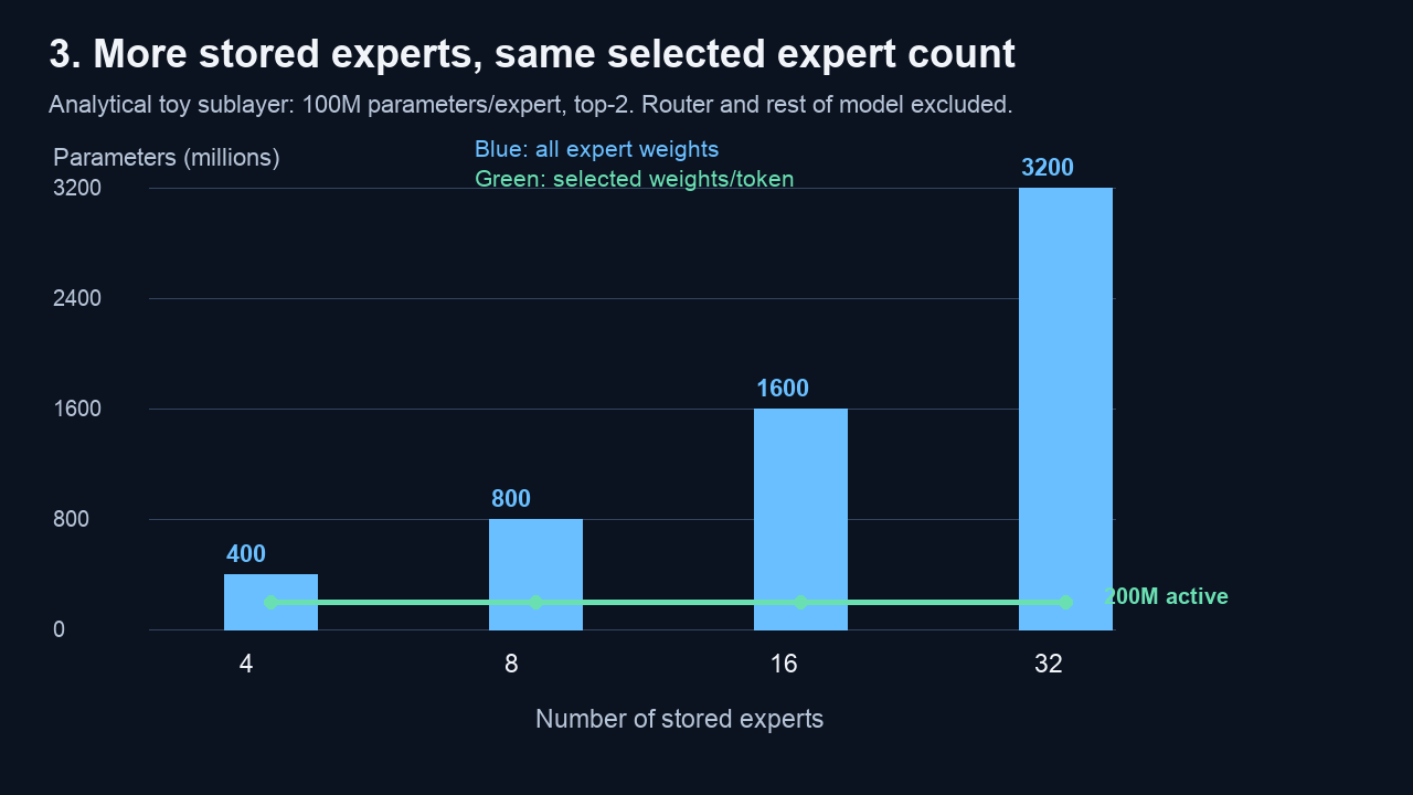
Analytical counts for equally sized experts with top-2 routing. The chart excludes router work, attention, and the rest of the model.

There are two independent knobs: how many expert functions exist, and how many each token evaluates. Increasing the first creates more choices. Increasing the second asks each token to do more expert work.

For a toy model with one routed layer:

total parameters  = shared parameters + E × parameters per expert
active parameters = shared parameters + k × parameters per expert

E is the number available; k is the number selected. For multiple routed layers, add each layer’s contribution. This is a simplified counting convention, not a formula for latency or literal weight bytes read.

Mixtral 8x7B provides a concrete example: its paper reports roughly 47 billion total parameters and 13 billion active parameters per token, with two of eight experts selected at each layer. Shared components explain why its name does not mean eight complete 7B language models copied side by side. Mixtral paper

6. The switches save work, but the workshops still occupy space

An idle expert still has weights. Later tokens may need it, so those weights must remain available. Keeping all weights in accelerator memory makes routing immediately executable; offloading introduces transfers and loading delays. Sparse activation therefore leaves a substantial storage requirement. Hugging Face’s MoE guide

For our eight-expert toy layer, two bytes per parameter gives:

stored expert weights = 8 × 100 million × 2 bytes = 1.6 GB
one token selects     = 2 × 100 million           = 200 million parameters

That is 1.6 GB in decimal units for expert weights alone. Attention weights, the router, activations, the KV cache, and runtime buffers add their own memory requirements.

Imagine a library. A reader consults two books, but the library still houses all eight. Consulting fewer books reduces the reader’s work. It does not shrink the shelves.

The analogy also exposes a second complication: many readers can collectively consult every book.

7. A batch can wake up every expert

Suppose four tokens select the following pairs:

A → E0, E2
B → E1, E2
C → E0, E3
D → E2, E3

Each token uses two experts. Across the batch, all four experts are active.

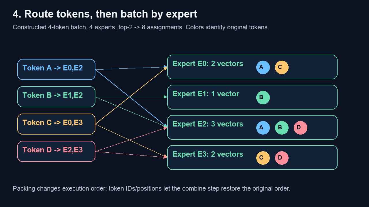
This is a separate invented batch. Colors track token identities while the runtime groups assignments by expert.

Count the assignments: E0 receives two; E1 receives one; E2 receives three; E3 receives two. There are eight assignments altogether, exactly four tokens times two choices.

Grouping vectors by expert lets the GPU reuse an expert’s weights across several inputs. But tiny or uneven groups can use the hardware poorly. Low-concurrency generation offers fewer vectors to group than a large prompt or a batch of many requests. Hugging Face guide, sparsity and serving discussion

Some implementations allocate a fixed capacity per expert. Overflow can skip assigned expert computation; padding unused slots wastes work and memory. Dropless approaches such as MegaBlocks use block-sparse computation to handle variable expert loads without dropping tokens. Capacity and overflow behavior depend on the design. MegaBlocks paper

This is why “two out of eight experts” cannot be turned directly into “four times faster.” Hardware sees batches, memory traffic, and kernels as well as the per-token selection rule.

8. How do the experts learn?

The experts begin as learned networks with random initial weights. Training uses prediction errors to adjust the model, including the router and expert functions. Selection directs learning opportunities: frequently chosen experts receive more examples. Jia-Bin Huang’s explanation, 16:37–17:27

Picture eight exercise books, but a student keeps practicing in only two. Those two fill up; the others remain nearly blank. A routing system can develop a similar imbalance.

Training methods address this with mechanisms such as noisy routing and auxiliary balancing objectives. The goal is to make useful use of the available experts while preserving prediction quality. Switch Transformers demonstrates a top-1 design and an auxiliary load-balancing loss; top-2 is one design choice among several. Switch Transformers

Every expert needs practice, but that does not mean every expert must process exactly the same number of tokens in every batch. Imagine a batch containing many similar token vectors. The router may favor the same two experts for most of them. Forcing equal token counts would send some vectors to other experts simply to fill their quotas, even when the router gives those experts lower scores. A balancing objective therefore encourages broader expert use while allowing some unevenness: experts should receive enough examples to learn, and routing should still help the model predict well.

Architectures also differ in what stays active. DeepSeekMoE introduces finer-grained routed experts and always-active shared experts. Any shared expert contributes work even when only a few routed experts are selected. DeepSeekMoE paper

9. When the experts live on different GPUs

So far, our arrows moved across a drawing. For a large deployment, those arrows may cross physical links.

Expert parallelism places different experts on different GPUs. A token vector must reach the device holding its selected expert; the resulting vector must return for combination. Splitting ownership reduces the expert weights each device stores and adds communication. MoE describes the model architecture; expert parallelism describes one way to execute it. NVIDIA’s expert-parallelism guide

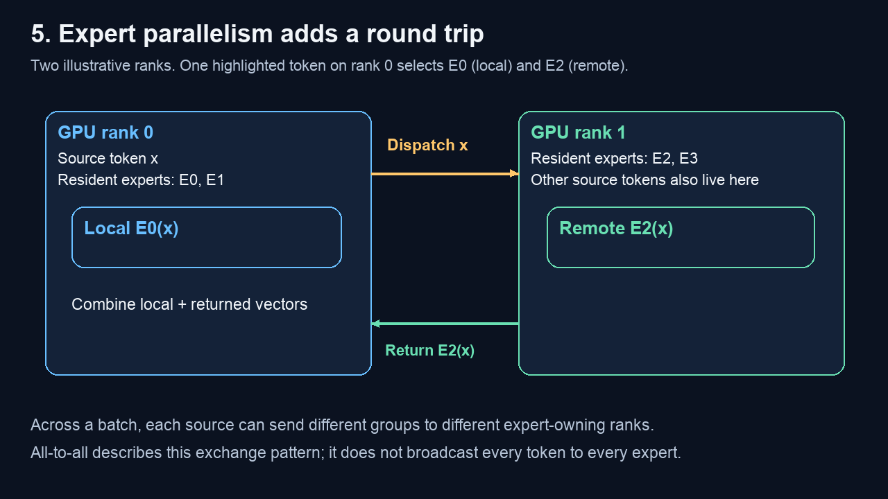
Separate placement example: E0 is local and E2 is remote. Only the remote assignment makes the illustrated round trip.

Now the workshops resemble buildings connected by roads. A short route to an idle building can work well. A congested road or an overloaded building can make the whole trip slow.

That is the practical bargain: more available learned capacity for limited per-token expert computation, paid for with storage, routing, and sometimes communication. Whether it improves latency or throughput depends on the actual model, workload, placement, and hardware.

Keep the original picture in mind:

contextual token vector
          ↓
   router selects a few experts
          ↓
   selected networks transform the vector
          ↓
   scale and add their outputs
          ↓
   one vector continues through the model

The wall can grow. Each token still lights up only a few switches. The engineering challenge is keeping those selected paths useful, balanced, and cheap enough to travel.

---

Reference videos and source notes

These videos provide further visual explanations:

• What is Mixture of Experts?
• Mixture of Experts (MoE), Visually Explained
• A Visual Guide to Mixture of Experts (MoE) in LLMs
• Mixture of Experts Explained Visually: How Trillion-Parameter Models Actually Work

The numerical examples and vector diagram are original teaching examples. Technical sources were checked on October 4, 2026. This article describes sparse MoE in Transformer language models; broader MoE formulations can also blend all experts. No performance benchmarks are claimed.